Forecasting Slow-wave Activity from EEG using FFT
Providing closed-loop, phase-locked neural stimulation often requires some degree of prediction or forecasting of the observed neural (i.e. EEG) data to account for software, hardware, or wireless transmission delays. Slow-wave activity (SWA; ~0.5-4 Hz) is a common target because of it characterizes non-rapid eye movement sleep (NREM; or ‘deep sleep’) and can be augmented or enhanced using transcranial, direct-current, or audio stimulation. There are a few notable approaches for detecting SWA:
-
Deep sleep maintains learning efficiency of the human brain disturbed SWA when it crossd a -30μV threshold in a 2-second window using a Butterworth filter (0.5–2 Hz, stop-band<0.1 and >10 Hz, stopband attenuation 20 dB, passband attenuation 0.1 dB) using LabVIEW. A human maintained watch of the electromyogram (EMG) to ensure stimulation was not cued if the subject was awake/aroused.
-
Auditory closed-loop stimulation of the sleep slow oscillation enhances memory identified the negative half-wave peak of slow oscillations (0.5–2Hz) in real-time using Spike2 software triggering stimulation (by default) at -80μV.
-
The shaky ground truth of real-time phase estimation builds on Real-Time Brain Oscillation Detection and Phase-Locked Stimulation Using Autoregressive Spectral Estimation and Time-Series Forward Prediction to, in brief, forward-predict signal phase based on an optimized signal passband (see Phastimate on Github). These papers and the one below (4) are concerned with faster, theta (4–9Hz) EEG data.
-
Continuous Phase Estimation for Phase-Locked Neural Stimulation Using an Autoregressive Model for Signal Prediction discusses the work in (3) and instead of using zero-phase filtering, applies a Butterworth filter in the forward-only direction. Phase prediction was performed using a Hilbert transform after applying an autoregressive model to fill in the predicted future filtered data. This method is wrapped into an OpenEphys module.
-
A Fast EEG Forecasting Algorithm for Phase-Locked Transcranial Electrical Stimulation of the Human Brain is a compelling response to (3,4) that finds phase estimation can be as accurate using a simpler approach. This method is expanded on below.
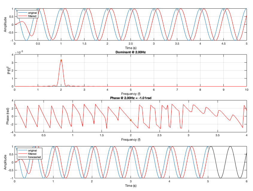
I find the approach in (5) the easiest software approach to phase estimation in an embedded system using C code. It uses a simple and straight-forward IIR filter along with a fast Fourier transform (FFT) that both have precedence in C (see KISS FFT, FFTW, or CMSIS DSP). Below is a prototype of the system implemented in MATLAB, which follows the simplified procedure of (5, Figure 1).

Row 1: Simulated 2Hz oscillation (blue) filtered using an IIR elliptical filter (0-5–4Hz, red). Row 2: Single-sided power spectrum of filtered signal deteremined by FFT. Row 3: Phase of filtered signal deteremined by FFT.
Row 4: Phase-shifted, forecasted signal (black).
Note, the forecasted signal has undergone an additional phase shift due to the filter design, which needs to be corrected (not shown). I discuss how to empirically derive the filter delay in the Mathworks Answers forum, Practical use of Phase Delay for IIR Filter on Pure Sinusoid. In brief, the phase delay can be adequetely modeled by a polynomial function. With this information, the forecasted signal can be used along with known system delays to cue phase-precise neural stimulation.
Simulating with Real Data
The Predict brain deep sleep slow oscillation has a database of labelled slow-wave data which I am using for testing. Building on the previous section, a forecasted (and phase-corrected) signal is actually not the ultimate goal: the goal is to know when a slow-wave will approximate a particular phase to be used in delivering phase-precise stimulation.
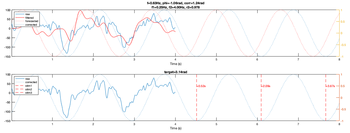
The composite phase delay described above (the offset of the original signal corrected by the phase shift of the filter) applies to t=0, not the where the original signal ends. Therefore, the phase at the end of the original signal—which is simulating a data buffer—needs to be calculated. From that, a phase difference between a target phase and the current phase can be converted into samples or time.
Below, the top row shows the raw data (4s of SWA), the filtered data (0.25–4Hz elliptical filter), along with the forecasted and corrected sinusoids. In this case, the FFT identified a dominant rhythm of 0.63Hz, and when overlaid with a phase-corrected cosine (bottom row), this matches reality. I chose a target stimulation phase of -π (i.e. the negative deflection) and plotted the next three stimulation opportunities based on the end of the raw data.

As noted at the end of the previous section, the only thing left to determine is if system/transmission delays would allow for stimulation to take place at one of the marked time points.
MATLAB Gist for first figure
Recent Comments
Archives
- April 2023
- January 2023
- November 2022
- May 2022
- March 2022
- January 2022
- December 2021
- April 2021
- December 2020
- October 2020
- August 2020
- July 2020
- March 2020
- February 2020
- January 2020
- December 2019
- November 2019
- October 2019
- January 2019
- December 2018
- November 2018
- August 2018
- July 2018
- April 2018
- March 2018
- November 2017
- October 2017
- February 2017
- October 2016
- August 2016
- July 2016
- November 2015
- October 2013
- February 2013
- January 2013
- August 2012
- July 2012
- June 2012
- May 2012
- April 2012
- February 2012
- December 2011
