Data Required to Detect and Forecast EEG Slow Waves
In a previous post, I explored a method of Forecasting Slow-wave Activity from EEG using FFT but did not treat its sensitivity. Mansouri et al. (2017) provide a sensitivity analysis for the 2–4Hz band, and here I perform a similar assessment for the 0.5–4Hz band with some changes that are more specific to slow-wave activity (SWA).
I am using the data from Predict brain deep sleep slow oscillation and will test the method only on the entries where “a slow oscillation of high amplitude started in the following second” (n=68,982). These data are 10s EEG recordings with a sampling frequency of 125Hz: “each sample represents 10 seconds of recording starting 10 seconds before the end of a slow oscillation.” Therefore, I used the 7-second mark to split training ‘training’ data from ‘test’ data.
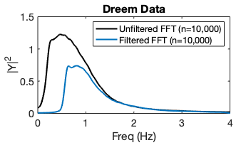
Fast Fourier transform (FFT) of Dreem data unfiltered and filtered (10s, 0.5–4 Hz).
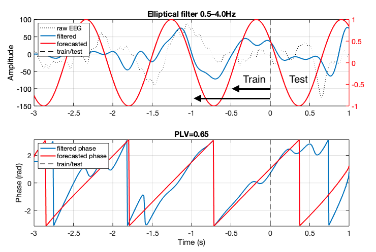
Single recording sample. Where t=0 is 7-seconds into the EEG recording sample from the Dreem dataset. This was done to keep keep the testing area consistent and assumes the SWA occurs around this mark, which was confirmed empirically. The ‘training’ area (left of t=0) was incremented by 0.5s (read more below) and the phase error was measured in the ‘test’ window (right of t=0). A phase locking value (PLV) was determined for the entire test window (1s).
Methods
Filtering data. The training and testing data wire extracted from the original 10s recording and filtered (the filter design for MATLAB is pasted below). These data were then split into training and testing data around the 7s mark of the original recording. Training data was swept from 0.5–3s in 0.5s increments. Test data was a 1s window following the training data.
f1 = 0.5; f2 = 4;[A,B,C,D] = ellip(10,0.5,40,[f1/fs*2 f2/fs*2]);EEG Forecasting. The dominant frequency and phase of the training data was determined using a FFT (see Forecasting Slow-wave Activity from EEG using FFT). No filter correction (i.e. delay) was applied because the phase comparison performed later is against filtered data. A phase comparison against raw data would be taking into account all frequency components—here, the target is SWA. Lastly, a forecasted signal is generated using the dominant frequency and phase (extended into the test window, t) using cos(2*π*frequency*t + phase).
Performance Metrics. Phase locking value (PLV; see Lachaux et al., 1999) is useful for determining if the phase of two signals are in sync, spanning from 0 for signals with no phase relation to 1 for phases that are completely aligned. It should be noted, PLV will still be high for signals that are phase-shifted. Phase error, as I present it below, is the unwrapped circular mean (using CircStat for MATLAB) from the training data to the test data on a sample-by-sample basis; therefore, the phase error is bounded from 0 (no error) to π (max error).
Results
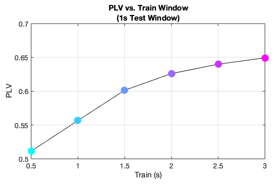
Mean phase locking value (PLV). As the training window increases, the PLV increases for the following 1-second test window. These results are consistent with Mansouri et al., Figure 5.
Mean PLV increases given more training data, which was expected. A training window of 0.5s can only contain a single oscillation for frequencies >=2Hz, thus the performance of the FFT algorithm will suffer for lower frequencies. With a 3s training window, the mean dominant frequency for all samples (n=68,928) was 1.16Hz (a period of 0.86s). However, this could be an effect of the selection criteria of the dataset (i.e. what defines a slow-wave). In any case, using a training window of less than 1s might result in poor performance, supported by the PLV results. An ideal tradeoff between the training window and PLV seems to be around 2s.
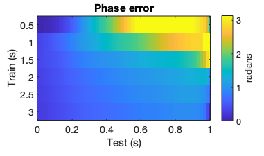
Mean phase error. Error is bounded bounded from 0 to π.
Mean phase error can be appreciated as the drift from a perfect phase forecast and is shown for an increasing test window. Practically, this is important because unless a system has zero transmission (e.g., hardware, software, wireless) delay, the forecasted phase will incur error over time. This accumulated error will affect the ability to accurately stimulate with phase-precision, likely resulting in poor experimental efficacy.
As expected, the phase error increased as the test window was extended. This is consistent with the result that PLV is also poor for small training windows. However, the phase error at a training window of 2s remains relatively low; at 0.5s the phase error is 0.95 radians or 54.43 degrees.
phase optimization
One disadvantage of the FFT method is that the phase derived from the transform applies to the entire data window. Therefore, it wasn’t suprising to find some ‘baseline’ phase error where the training data meets the test data, which was true on a number of instances I inspected. In the first figure above (bottom row), this would be the difference between the red and blue lines at the dashed line (t=0). My hypothesis was that using the tail-end of the training data to ‘optimize’ the phase leading into the test area would reduce the phase error. I tested this using a 2s training window and optimized (i.e. corrected or ‘re-aligned’) the phase based on the last 0.25s of the training window. This assumes access to a Hilbert transform to compare the instantaneous phase of the forecasted versus real filtered waveforms.
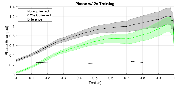
Non-optimized vs. optimized mean phase error. Shaded areas represent the 95% confidence bounds across all samples (n=10,000). The phase difference (dotted) is non-optimized minus optimized data.
These results confirm my hypothesis and demonstrate that the phase gathered from the FFT is optimized for the whole 2s window, not the tail end. Since this is a signal forecasting (rather than signal matching) exercise, optimizing the phase shift by the ‘most recent’ data appears to provide an advantage. Why not only use the 0.25s window for prediction then? The FFT and Hilbert transform will have issues on small data snippets, which was demonstrated by the PLV suffering from a small training window above. Another—perhaps obvious—conclusion from these data is that minimizing the latency to stimulation (represented here on the x-axis) is a critical for accuracy. Theoretically, the need for forecasting is eliminated with zero latency, and becomes more important as time increases.
Conclusion
These results reinforce the idea that a long training window leads to better frequency and phase estimation, ultimately providing better forecasting accuracy. Some caveats should be addressed. Firstly, a slow oscillation (sometimes called a ‘delta wave’) is loosely defined and there is some controversy over the best filter to use and the physiologic relevance of the identified oscillations (see Spontaneous neural activity during human slow wave sleep). If slow oscillations or periods of SWA are transient—perhaps only encompassing a period of 2s or less—a more eager detection method would need to be used that is focused on the detecting the onset of the slow wave. Secondly, the results shown here are dependent not only on the filter selection, but also on the source data; surely, PLV and phase error will be different for other data sets, but it could be assumed the trends will remain the same. Finally, since SWA is by definition oscillatory, the FFT is well-suited to detect and forecast the underlying frequency and phase characteristics. Indeed, EEG is said to be locally stationary (i.e. exhibits oscillatory characteristics) in short time windows, and therefore, non-adaptive models are suitable for forecasting (see Chen et al., 2011). However, I show that a simple optimization step enhances the performance of the algorithm which suggests the oscillation is not completely uniform over time, or at least, not within my sample window. I do suspect that a machine learning approach might be more accurate for specific applications (e.g., the Dreem dataset used here), but then again, might suffer when generalized across subject conditions or species.
In conclusion, given a 2s data buffer and computation/transmission delays of less than 0.5s total, closed-loop neural stimulation using a FFT method with a phase optimization step is desirable for its simplicity, portability, and performance.
