Cross Correlation Normalization in MATLAB
Cross Correlation Primer
A cross correlation measures the similarity of two signals over time. It’s an important analytical tool in time-series signal processing as it can highlight when two signals are correlated but exhibit some delay from one another.
For instance, imagine that you are talking with a friend in Tokyo while making a simultaneous recording from the microphone of your phone (in the States), and the headset of their phone. Both signals will represent your voice, but will not be correlated because of the delay: the local recording will be at “How are you?” while the distant recording will be at “Hello!”. A cross correlation takes two time series signals and sweeps them across each other to determine exactly when, and to what extent the signals are correlated in time. In this case, a cross correlation will reveal a perfect correlation of the signals, albeit with a delay.
In neural physiology, cross correlation is often used to determined the relationship between two phenomena. It could reveal that one neuron always fires before, or after another one. Or, it may expose how the firing of a neuron relates to local field potential activity.
Cross Correlation in MATLAB
The MATLAB xcorr function will cross correlate two time-series signals. The MATLAB documentation offers a good example using two sensors at different locations that measured vibrations caused by a car as it crosses a bridge. What I want to show here is the functionality of using the ‘coeff’ scale option to normalize the cross correlation. By normalizing, the cross correlation ignores the magnitude disparity of the source signals.
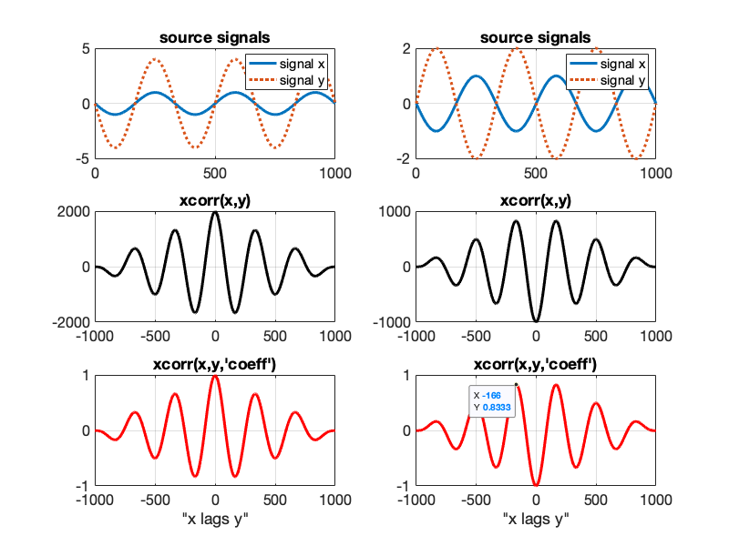
(right) The two source signals are perfectly anti-correlated in time and differ in magnitude.
(left) The two source signals are correlated in time and differ in magnitude.
The raw cross correlation (middle row) scales the y-values based on the magnitude of the source signals. This may be interpreted as, the signals on the left are correlated to a higher degree than the anti-correlated signals on the right.
So why use normalization? One case might be where the source signals are coming from uncalibrated sensors (i.e., the phase information is accurate, but the magnitude is not). Here, you are only interested in whether the phase of the signals is correlated in time.
Interpreting “x lags y”
The left column cross correlation tells you that the maximum correlation occurs when signal x lags signal y by 0 samples. This is simply because the two signals are perfectly correlated in time. In the right column, I included a data tip showing the greatest positive correlation of the “perfectly” anti-correlated source signals: it occurs where signal x lags signal y by -166 samples, but only reaches a positive correlation of 0.8333. Even though the signals have the same frequency, the cross correlation will never reach 1 because as the time lag is increased, signal a will overlap less with signal b. Note, these signals alway reach an identical positive correlation at +166 samples because the source signals are symmetrical.
How-to Normalize
The normalization procedure is rather straight forward. I’ve appended a YouTube video that explains cross correlation and normalization in mathematical detail. In brief, the ‘coeff’ method can be bootstrapped using the following code:
acor_norm = xcorr(x,y)/sqrt(sum(abs(x).^2)*sum(abs(y).^2));
