Have you ever wondered: is my filter working? In neurophysiology, we are often faced with mashing together data, and in the process, sampling rates and filter settings can get lost. You are always one parameter away from interpreting a beta oscillation (13-30 Hz) as a delta oscillation (1-4 Hz), which can lead research far from the truth.

To check whether a filter is working properly, a ground truth local field potential (LFP) or “wideband” signal should be used, where the timing and frequencies are known. Here, I have created an LFP generator with control over all aspects of timing, frequency and amplitude.

Ground Truth LFP M-file

The LFP generator combines sinusoids based on the input parameters to generate a single waveform as the output. The variable, t, represents the time course and is the same length as the lfp.

An Example

My primary reason for creating this was to test if the spectrogram function I use is accurate in both the time and frequency domain. For instance, most analyses require my filter to be non-causal (i.e., centered on the input phenomena with zero-lag). Here is an example of how to use groundTruthLFP.m.

The LFP I constructed is 10 seconds long with a sampling rate of 1,000 Hz. The first frequency I added was at 4 Hz, from 0-10 seconds with unity amplitude. The third frequency was 30 Hz, from 0-5 seconds with an amplitude of 3. Then, Iran the lfp through my spectrogram function to see if the output matches the signal I designed.

Altogether, it looks really good. You can get a feel for the rolloff properties of the filter and causality. Most importantly, the frequencies and timing are spot on.

Caveats

This function does not pay any special attention to the phase of the input signal. It begins all sinusoids at the time specifed in oscillationOnOff at 0π. Therefore, waves of similar frequency will have phase interactions that may lead to noticeable segments of constructive and destructive interference in the output. For example, notice how the following example has nearby input frequencies, resulting to a non-trivial spectrogram.

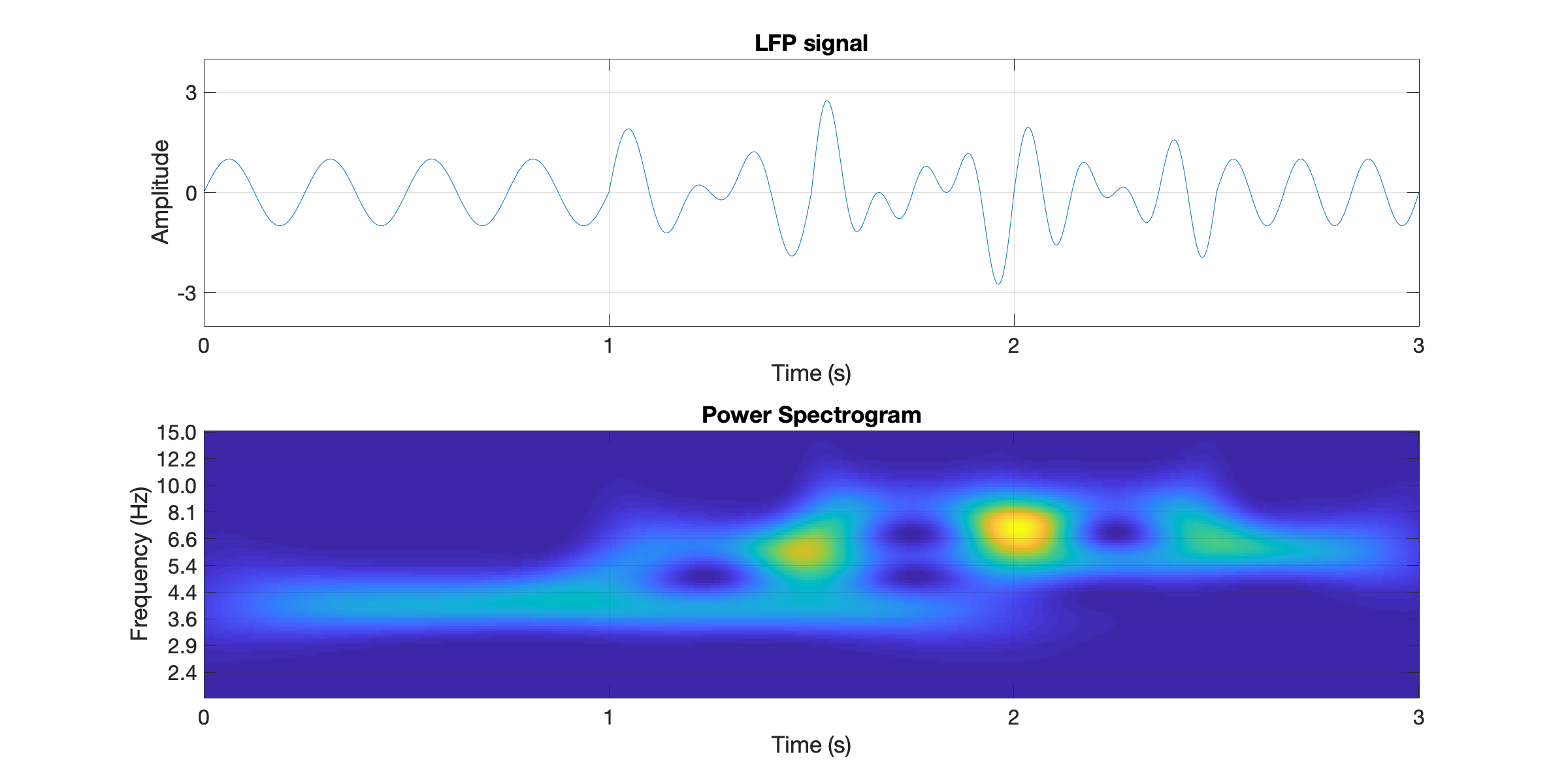
This example highlights just one of considerations when analyzing LFPs from the brain, where signals arriving from different brain structures may have no phase coordination, but are ultimately summed together. That is, the fun.