On Optimal Timestamps for Bio-loggers
Bio-loggers are optimized for physical size, power, memory, and cost constraints—and probably in that order. Here I discuss memory optimization, first highlighting the fact that storage capacity affects component size and write frequency affects power consumption. This applies to non-volatile NAND flash storage which is common in 1-2Gb capacities and preferred [over the nearly endless storage of a micro-SD card] for its low-power performance (which is a design consideration itself, see Low Power Showdown: uSD Card Sleep and Write Current Draw). The other constraints are operational:
-
The sensor system (e.g., bio-logger) can have a power failure at any time, even while writing data, and prior data remains intact.
-
The memory structure itself is widely interpretable, can be read directly from the memory module itself, and processed by standard toolsets (e.g., MATLAB, Python, C).
I treat these constraints with a focus on how to properly build an efficient time-series memory structure for low-power devices that sleep or irregularly sample multisensor data.
A File Primer
Developing (or using) a File System is typical when using something like a micro-SD card because it is robust, supported across platforms, and speedy to implement. However, if memory is limited, a file system has some disadvantages. For example, files themselves are not ideal for multisensor data that has an undefined structure or sampling scheme. Files also break constraint #1, such that the entire file system is susceptible to corruption if the system is powered down while writing new data or performing file system maintenance; some of these issues are discussed in How do I protect SD card against unexpected power failures?.
One architectural consideration from a file system is the use of an independent directory to specify data type (or filename), data location, data length, and potentially metadata like a timestamp. This is an efficient way of storing data but has distinct drawbacks. Firstly, if the directory is corrupted, the data is likely unrecoverable. Secondly, files typically have poor temporal resolution (or version history). Related to this, it can be really inefficient to work with files because they often have to be worked on as a whole, or in chunks, creating a large read and write overhead on relatively small or simple additions to memory.
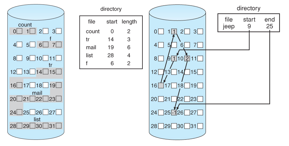
Examples of file system architectures using a directory or “lookup table”. Contiguous (left) and linked (right) allocation of disk space. Source.
Specific Use Case
While contiguous memory allocation is attractive for its efficiency, the separation of data from its type, length, and time of entry breaks design constraints while requiring some degree of file management software to be built and maintained. Let’s consider the sensors system (“bio-logger”) below, which might be implanted in an animal.
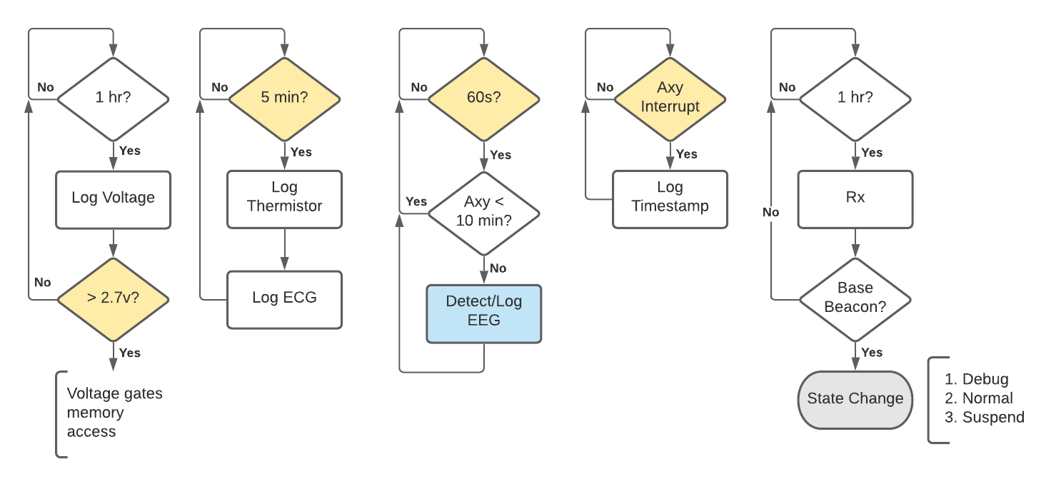
Bio-logger (i.e. multi-sensor) timing and interrupt design. Left to right: Every hour the system voltage is logged which “gates” other functions that access the memory module (to mitigate low-voltage errors). Every 5-minutes a thermistor logs body temperature and an electrocardiogram (ECG) waveform is sampled and logged. Every 60-seconds the accelerometer (Axy) status is checked and gates a detection and logging routine for electroencephalography (EEG). The Axy status is logged using an interrupt, triggered by a movement threshold. Finally, the system checks for a base station (Rx) as a way of changing state. When these functions are not being performed, the system is sleeping (in a “forever” loop).
In the described system, it can be appreciated that data of different types and lengths might need to saved at different time intervals—some which are regular, and some (e.g., accelerometer) that might occur stochastically. This use case illustrates the problem with using a file system: should a single accelerometer timestamp be placed in one file? How are timestamps recorded for all events? The case is further complicated by the fact that ECG and EEG waveforms will consist of many data points, potentially at different sampling rates.
Simple Memory Structures
Since file management poses a number of challenges for multi-sensor, irregularly sampled data, it is worth considering other ways managing data without sacrificng the benefits of a contiguous data stream. One compromise is to augment the directory function by placing descriptive headers ahead and/or behind data segments (see figure). The header might contain what type of record is upcoming, its length, time recorded, sampling rate, etc.

Record Sequential File with Variable Length Records. Source.
The issue with a record header and variable record length is that reading the nth data record depends on the nth-1 header being intact and correct. That is, if looking purely at the byte stream, there is nothing that definitively delineates the header from the record, and data integrity requires all headers to be descriptive and accurate. Imagine, for some reason, a data record writes 249 data points instead of 250; this could affect everything downstream of that data segment.
Ideas on Identifying Headers vs. Data
There are a few options that can help get around the pitfalls of the sequential dependency. One method would be to use a fixed-length record system, but this does not have a clear implementation for records of different types. Another method would be to embed a small (e.g., 4-bit) checksum in the header itself. The checksum sums the useful bits in the header and is itself, the modulo of that sum. This would not provide a perfect delineation between header and data, since there is some likelihood that sensor data could meet the criteria of a header-with-checksum, but it is highly unlikely and could be caught with some logic on the interpreter. This is essentially a more robust parity check on the header.
The last option is to use fixed data lengths for header and data, but use the most- or least-significant bit as a type-flag for header or data. Although odd-numbered data packets are common where parity is involved, it plays poorly with two’s complement (i.e. signed) data.
An Optimal Solution
Given that files have several layers of overhead and that variable-length headers or data can be problematic if power is cut off or data becomes partial, an ideal solution might use inline, fixed-length headers and data as a compromise. I describe a blended approach that is relatively failsafe and efficient for an embedded, time-based sensor system.
Bio-logging Header and Data Format
The maximum size of my sensor data is 24-bits and will comprise more than 90% of my data records. Therefore, there is not much to gain from having variable record sizes, even though some sensors only record 12-bit data. I am choosing to have an 8-bit header attached to each data record, for a total of 32-bits in each segment; this is the inefficient compromise for having every single piece of data be identifiable without a distant lookup table has only a slight dependency on sequential records, as explained below.
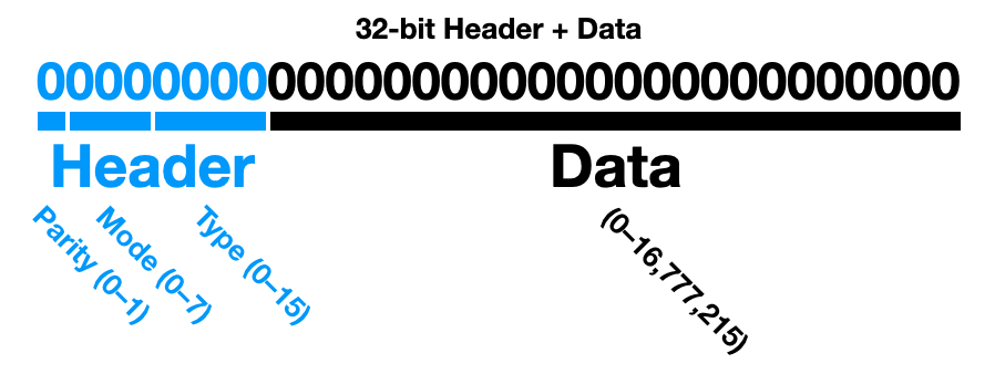
32-bit Data + Header. 24-bits of data is preceded by an 8-bit header with slots designated for a Parity bit, 3-bits for a system Mode, and 4-bits for the data Type.
Justification. Should the starting location of the data ever be lost, the Parity bit makes it possible to—by brute force—recover where data segments are located by scanning for a parity match at 32-bit intervals. The 3 Mode bits (8 options) are meant to encode system “state,” which could be used to delineate debugging, calibration, and deployment status, or set a flag as a low-voltage warning or mark potentially corrupted data. The 4 Type bits (16 options) set the data (or sample) type, such as temperature, accelerometer (Axy), ECG, or EEG sample. Taken together, Mode and Type should be defined in a table that is versioned alongside the codebase.
Implementing Timestamps. Firstly, recording a timestamp with each sample is a significant waste of memory. Secondly, even 32-bits can only encode millisecond timestamps for 49 days from when the device was turned on; this is inherently limiting to the system. The proposed solution—which fits into this 32-bit architecture—is to reserve the first bit of Type for the following:
-
Type[0] = 0 is Absolute Time: Seconds since the device was turned on.
-
Type[0] = 1 is Relative Time: Milliseconds since the last Absolute Time was recorded.
This scheme eliminates the burden of recording milliseconds over long durations but enables millisecond precision where needed. 24-bits of seconds can record 194 unique days of timestamps, whereas 24-bits of milliseconds can record 4.66 unique hours of timestamps. This imposes one necessary criterion of the system: that one record of Absolute Time be made before 4.66 hours of Relative Time records have accumulated.
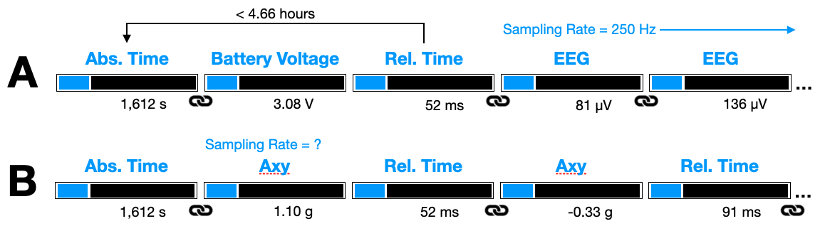
Examples using Absolute (Abs) and Relative (Rel) Time types. (A) Absolute time is recorded with a battery voltage (linkage symbol). Relative time is recorded prior to the first EEG data type, which has a fixed sampling rate, thus Relative Time entries can be skipped for the subsequent stream of EEG data. (B) Absolute time is linked to the first Axy data and Relative Time for thereafter.
A few notes on the above examples, which are meant to illustrate the flexibility of the timestamping scheme but might be implemented differently in practice. Linkages from time types to other types (e.g., EEG, Axy) would need to be inferred from the codebase, and should therefore be thought of as “rules” which the data interpreter would need to built into the decoding logic. (B) can be assumed to have a rule in place that prepends an Absolute Time if data has not been logged for n-minutes, otherwise, it prepends a Relative Time. These rules should be simple (i.e. minimal logic) and include some redundancy to perform sanity checks.
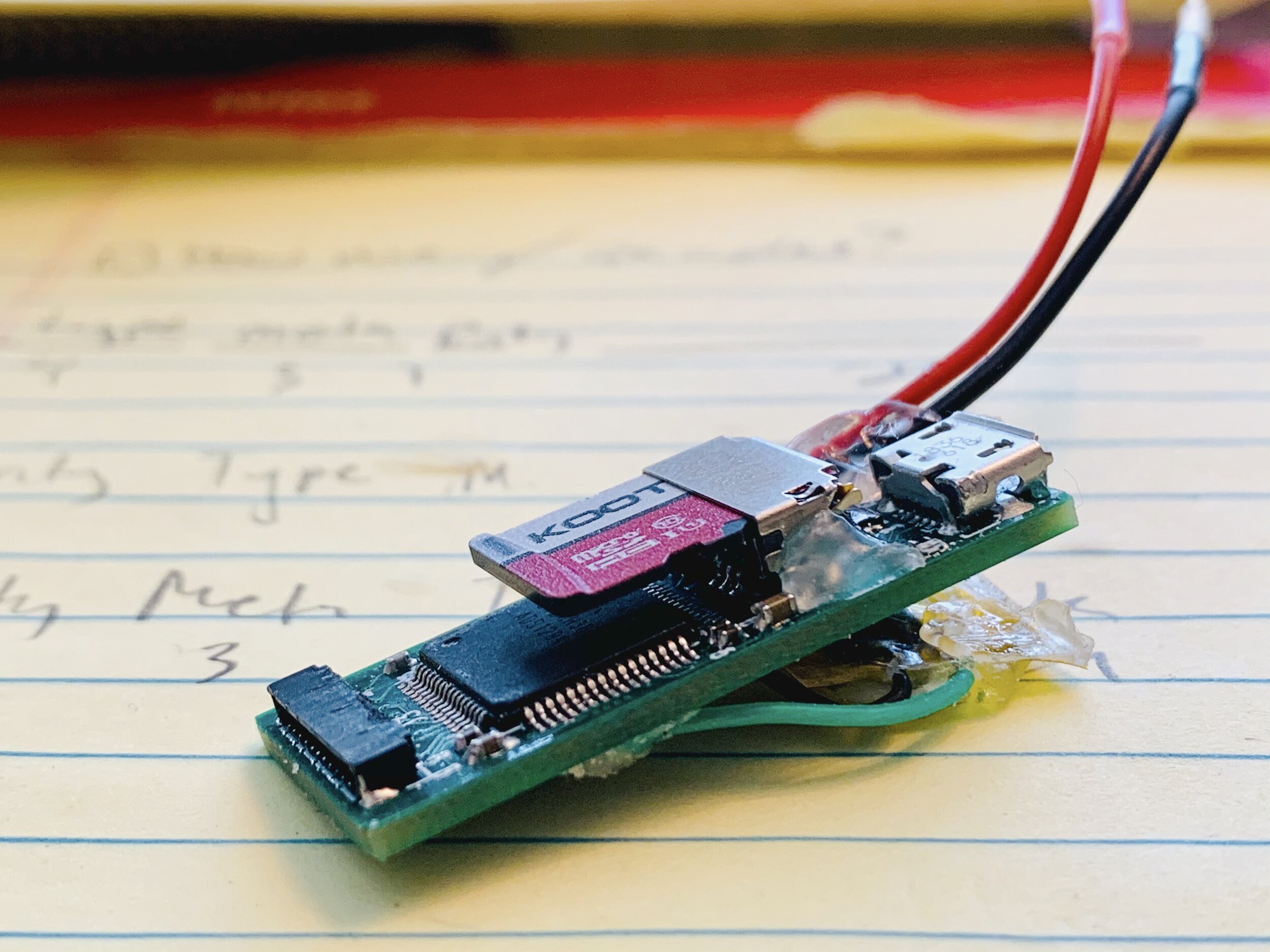
Bio-logger prototype based on a SAMD21G18A microcontroller and the ADS129X from Texas Instruments.
Conclusion
There is no perfect solution to data management; it is all a compromise, but those compromises need to be guided by system and operational constraints. Consider the bio-logger shown here: while the micro-SD was a rapid solution with clever physical placement, my recording constraints were such that the battery being used could only fill a few gigabytes of storage if running continuously. Therefore, I could explore other solutions that might be smaller and more power-efficient (e.g., NAND flash). I provide a simple calculator below which may be a starting point for your own application.
You can find more calculators and details about bio-logger architecture on my Project Wiki and the project itself here.
