Equalizing Sampling Rate for 1-D Correlations in MATLAB
We often have two signals with different sampling rates that we want to correlate. One example is when we want to correlate local field potential (LFP) activity of a neural signal to some average spike rate of a neuron. Our LFP signal is recorded at 24 kHz, but the spike density estimate (SDE) we create from individual spike timestamps is given an artificial sampling rate of 1 kHz. End-to-end, the LFP and SDE are potentially correlated, but to operate on those as variables in MATLAB they need to be the same length.
In this function, we use 1-D interpolation to force d1 data into the length of d2 and call that d1new. Ideally, your d2 data has the higher sampling rate so that d1 is being ‘upsampled’ instead of ‘downsampled’.
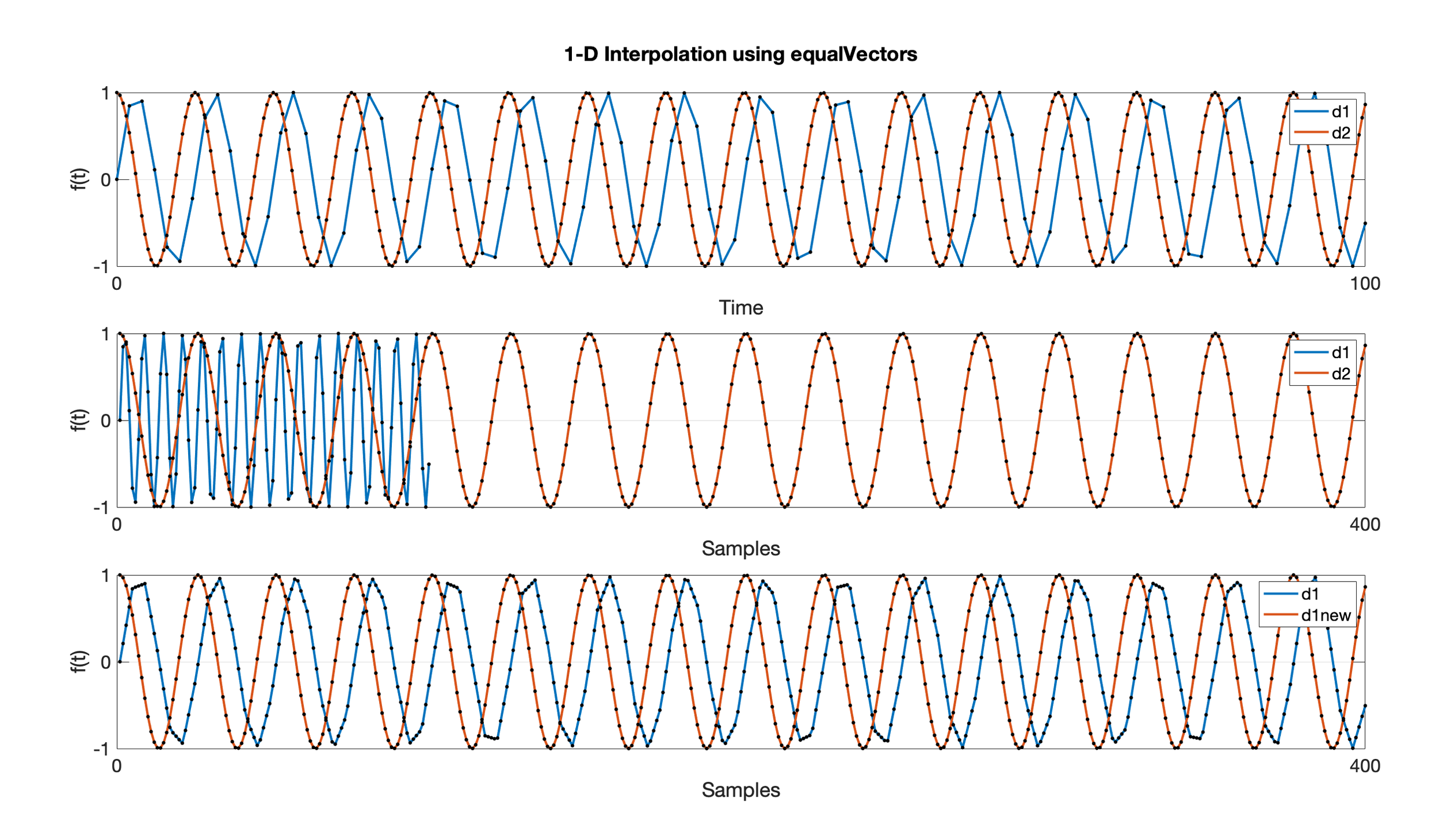
Consider two signals (d1 and d2) where f is either sin() or cos() and the time variable t is 0-100s, but each t has a different sampling rate.
t1 = linspace(0,100,100); % 0-100s, 100 points, 'low' sampling ratet2 = linspace(0,100,400); % 0-100s, 400 points, 'high' sampling rated1 = sin(t1);d2 = cos(t2);d1new = equalVectors(d1,d2);The top plot shows the signals overlaid in Time with each point from t marked in black. The middle plot highlights that when plotted by Samples, the two signals are unequal in size. The bottom plot shows how 1-D interpolation through equalVectors and the d1new variable equalize the vector lengths, thereby making a correlation possible.